Kernel PCA for image modeling
HTWG Konstanz, Brauneggerstr. 55, D-78462
Max-Planck-Institute for Biological Cybernetics, Spemannstr. 38, D-72076
· Kernel Principal Component Analysis
· Single-frame superresolution using iterative KPCA
Kernel Principal Component Analysis
We investigate the analysis of images based on kernel PCA (KPCA). Memory and time complexity are, however, major obstacles for applying KPCA to huge image databases. The generalized Hebbian algorithm (GHA) provides an efficient implementation of linear PCA with smaller demands on memory complexity. Accordingly, we study the transfer of this property to KPCA by kernelizing the GHA.
|
|
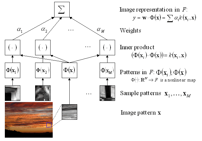
The basic idea of KPCA for image analysis is to nonlinearly map
the data into a Reproducing Kernel Hilbert Space (RKHS) F and then
perform linear PCA in F. The architecture of KPCA for the extraction of
the first principal component is depicted in Fig. 1. A patch of a natural image
is fed into the KPCA analyzer. A nonlinear map ![]() is then applied to map the input into the RKHS F,
where the inner product with the principal axis w is computed. These two
operations are in practice performed in one single step using the kernel
function
is then applied to map the input into the RKHS F,
where the inner product with the principal axis w is computed. These two
operations are in practice performed in one single step using the kernel
function ![]() . By expanding the
solution w as a linear combination of mapped samples, KPCA indirectly
performs PCA in F only based on the kernel function.
. By expanding the
solution w as a linear combination of mapped samples, KPCA indirectly
performs PCA in F only based on the kernel function.
In the original
KPCA formulation, the combination coefficients are computed by diagonalizing
the Gram matrix ![]() for all sample
patterns, which is prohibitive for natural images due to memory complexity. As
a nonlinear extension of the Hebbian algorithm, the Kernel Hebbian
Algorithm (KHA) estimates them iteratively based on the correlation between the
mapped patterns
for all sample
patterns, which is prohibitive for natural images due to memory complexity. As
a nonlinear extension of the Hebbian algorithm, the Kernel Hebbian
Algorithm (KHA) estimates them iteratively based on the correlation between the
mapped patterns ![]() and the system
output y in F, which can be efficiently computed based on kernels. This
relieves the burden of working directly in a possibly very high-dimensional
RKHSs and storing the whole gram matrix.
and the system
output y in F, which can be efficiently computed based on kernels. This
relieves the burden of working directly in a possibly very high-dimensional
RKHSs and storing the whole gram matrix.
Download matlab code containing the KHA and a toy example.
|
|
|
|
a |
b |
|
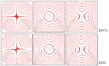
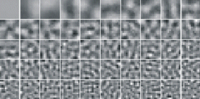
Fig. 2 shows preliminary results: a toy problem: two-dimensional data (scattered black dots) overlaid with the contours of three principal components (induced by polynomial kernel) obtained with KPCA and KHA, respectively (3,000 iterations for KHA); b natural image analysis application: preimages of 50 principal components (induced by Gaussian kernel) obtained from the KHA (40,000 image patches, 100 iterations). |
|
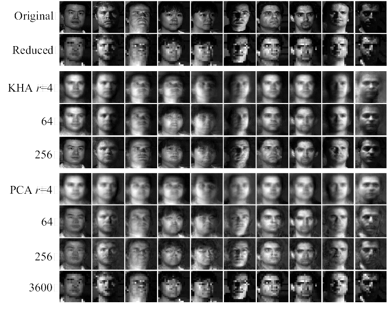
Figs. 3 and 4 show applications of the KHA to image super-resolution. The problem is to reconstruct a high-resolution image based on a low-resolution image. It requires prior knowledge which in our case will be provided by the kernel principal components of a representative dataset of high-resolution image patches. To reconstruct a super-resolution image from a low-resolution image which was not contained in the training set, we first scale up the image to the same size as the training images, then map the image into the F, and project it into the KPCA subspace corresponding to a limited number of principal components. This reconstruction in F is projected back into the input space by preimage techniques.
|
Fig. 3 Face image super-resolution based on PCA and KHA using a Gaussian kernel using varying numbers of principal components. 5000 (60 by 60)-sized face images were used to perform linear PCA and KHA. The test images were subsampled of a 20 by 20 grid and scaled up to the original scale by turning each pixel into a 3 by 3 square of identical pixels, before doing the reconstruction. |
|
|
|
|
a |
b |
|
|
|
|
c |
d |
|
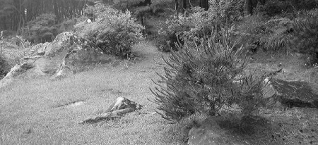
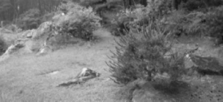
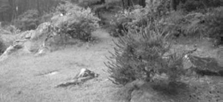
Fig. 4 Examples of natural image super-resolution. (12 by 12) image patches are used for training the KHA. For a realistic natural image super-resolution, only high-frequency components of image were reconstructed which are then super-imposed on the bicubic interpolation. The low-resolution input image is then divided into a set of (12 by 12)-sized windows each of which is reconstructed based on 200 principal components. The problem of this approach is that the resulting image as a whole shows a block structure since each window is reconstructed independently of its neighborhood. To reduce this effect, the windows are configured to slightly overlap into their neighboring windows: a. original image of resolution 284 by 618, b. low-resolution image (142 by 309) stretched to the original size, c. bi-cubic reconstruction, and d. KHA reconstruction. |
|
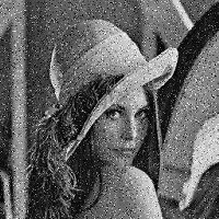
Fig. 5 shows applications of the KHA to image denoising. No clean training images are required. Instead, it is assumed that the noise mainly contaminates the kernel principal components (KPCs) with small eigenvalues. Thus, a truncated KPC expansion of the noisy image leads automatically to a denoising effect. The KHA is trained and tested on the same data set.
|
|
|
|
|
a |
b |
c |
|
|
|
|
|
|
d |
e |
|
Fig.5 Denoising examples. The training data for KHA were obtained by sampling noisy input images at regular intervals. Overlapping windows are averaged in the reconstruction. a. original Lena image, b and c. noisy images generated by adding Gaussian noise (SNR: 7.72dB) and Salt-and-pepper nise (SNR: 4.94dB), respectively, and d and e: denoised images of b and c based on KHA (SNR: 14.25dB and 12.71dB, respectively). |
||
